Exponentials

What is an Exponential?

An exponential is a power, otherwise known as an index.

\[ a^x \]

A base number \(a \) is raised to a power \(x \), the exponent.

Example

\(5^3\) has base 5, exponent 3.

\[ 5^3 = 5 \times 5 \times 5 = 125 \]

The inverse of an exponential function is the logarithmic function.

If \(y = a^x\), then \(x = \log_a y\).

Exponential Equations

To solve an exponential equation, take logs of both sides to the same base.

Scientific calculators usually have buttons for:
log (base 10) and ln (base \(e = 2.71828\ldots\)).

Example

Method 1: Using Logarithms

\[ 4^x = 64 \] Take logs: \[ \log(4^x) = \log 64 \] Bring the power down: \[ x\log 4 = \log 64 \] Solve: \[ x = \frac{\log 64}{\log 4} \] Since \(64 = 4^3\): \[ x = 3 \]

Solution: \(x = 3\).

Method 2: Without Logs

\[ 4^x = 64 \] Rewrite with base 2: \[ 4 = 2^2,\qquad 64 = 2^6 \] So: \[ 4^x = (2^2)^x = 2^{2x} \] The equation becomes: \[ 2^{2x} = 2^6 \] Equate indices: \[ 2x = 6 \] \[ x = 3 \]

The Natural Base \(e\)

The natural base \(e\) uses Euler’s number \(e = 2.71828182\ldots\)

\(y = e^x\) has the special property:

\[ \frac{d}{dx}(e^x) = e^x \]

The inverse of \(y = e^x\) is \(x = \ln y\).

Graphing Exponential and Logarithmic functions Excel – Exponential/log graphs

Growth Functions

A growth function is one where the output increases rapidly.

Example

£100 is deposited at 12% per annum.
Show that \(A(n) = 100 \times 1.12^n\).
Then find the amount after 10 years.

Building the Compound Interest Formula

\[ A(0) = 100 = 100 \times 1.12^0 \] \[ A(1) = 100 \times 1.12 = 100 \times 1.12^1 \] \[ A(2) = (100 \times 1.12)\times 1.12 = 100 \times 1.12^2 \] \[ A(3) = (100 \times 1.12 \times 1.12)\times 1.12 = 100 \times 1.12^3 \] \[ A(n) = 100 \times 1.12 \times 1.12 \times \dots \times 1.12 \]

(with \(n\) factors of \(1.12\))

\[ A(n) = 100 \times 1.12^n \]

Evaluating the Formula

\[ A(n) = 100 \cdot 1.12^n \]

Find \(A(10)\):

\[ A(10) = 100 \cdot 1.12^{10} \] \[ = 100 \cdot 3.10584820834420916224 \] \[ = 310.584820834420916224 \] \[ \approx 310.58 \]

There is £310.58 in the account after 10 years.

The account growth looks like this:

Example

A factory targets 1.5% growth per year.
Production in 2003: 18000 units.
Production in 2005: 18515 units.
Was the target met?

Expected Output

\[ \text{Expected growth factor} = 1.015^2 = 1.030225 \] \[ \text{Expected production} = 18000 \cdot 1.030225 = 18544.05 \]

Actual Output

\[ \text{Actual} = 18515 \]

The actual production is slightly below the expected value.

Comparison & Conclusion

\[ 18515 \;\lt \; 18544.05 \]

The expected output was not reached.

Target not met.

Decay Functions

A decay function is one where the output decreases rapidly.

Example

12,000 gallons of oil are spilled.The clean up crew manage to clean 60 % of the oil each week.
a) How much oil is left after 1 week ?
b) How many weeks of cleaning are needed until only 10 gallons remain?

Since 60% is cleaned each week, 40% of the oil is left

\[ A(t) = 12000 \times 0.4^t \]

\[ A(1) = 12000 \times 0.4^1 = 4800 \]

After 1 week of cleaning there is 4,800 gallons of oil left.

\[ 12000 \cdot 0.4^t = 10 \]

Step 1: Isolate the exponential

\[ 0.4^t = \frac{10}{12000} \] \[ 0.4^t = \frac{1}{1200} \]

Step 2: Take logs of both sides

\[ \log(0.4^t) = \log\left(\frac{1}{1200}\right) \] Bring the power down: \[ t \log 0.4 = \log\left(\frac{1}{1200}\right) \]

Step 3: Solve for \(t\)

\[ t = \frac{\log\left(\frac{1}{1200}\right)}{\log 0.4} \] \[ t \approx \frac{-3.07918}{-0.39794} \approx 7.74 \]

Solution: \(t \approx 7.74\) weeks.

Half Life

The decay of a radioactive source is given by:

\[ N = N_0 e^{-\lambda t} \]

where N is the number of radioactive atoms present at time t , λ is the transformation decay constant and N_o is the original starting value.

The half-life of carbon-14 is 5,730 ± 40 years and is used for radio carbon dating

Example

Find the decay constant \(\lambda\) of Carbon 14.

\[ N = N_0 e^{-\lambda t} \] Substitute \(t = 5730\) (the half‑life): \[ \frac{N}{N_0} = e^{-5730\lambda} \] Since after one half‑life the amount halves: \[ \frac{1}{2} = e^{-5730\lambda} \] \[ \ln\!\left(\frac{1}{2}\right) = \ln\!\left(e^{-5730\lambda}\right) \] Using \(\ln(e^x)=x\): \[ \ln\!\left(\frac{1}{2}\right) = -5730\lambda \ln(e) \] Since \(\ln(e)=1\): \[ \ln\!\left(\frac{1}{2}\right) = -5730\lambda \]

\[ \lambda = \frac{\ln\!\left(\tfrac{1}{2}\right)}{-5730} \] \[ \lambda = \frac{\ln\!\left(\tfrac{1}{2}\right)}{-5730} \] \[ \lambda = 0.0001209 \] \[ \lambda \approx 0.00012 \]

Log–Linear Graphs

Log scale on the y-axis only

If a graph has a logarithmic y-axis but an ordinary x-axis, then a straight line \(\log y = (\log b)x + \log a\) confirms a relationship of the form \(y = ab^x\).

If \(y = ab^x\) then \(\log y = \log a + x\log b\).

This is because of the log laws.

\[ y = a b^x \] Take logs of both sides: \[ \log y = \log(a b^x) \] Use the product rule: \[ \log y = \log a + \log(b^x) \] Bring the power down: \[ \log y = \log a + x \log b \] Rearranged into straight‑line form: \[ \log y = (\log b)\,x + \log a \]

Compare with \(Y = mx + c\), where \(Y = \log y\), \(m = \log b\), \(c = \log a\).

Example

Find the equation of the graph below in the form \(y = ab^x\).

The points (0,2), (2,4), (6,8), (10,12) lie on this graph.

So \(c = 2\), \(m = 1\).

\[ \log_2 y = x + 2 \]

Thus, comparing with the straight‑line form

\[ \log_2 y = (\log_2 b)\,x + \log_2 a, \] we identify: \[ \log_2 b = m = 1 \] \[ b = 2^1 = 2 \]

Likewise:

\[ \log_2 a = c = 2 \] \[ a = 2^2 = 4 \]

Putting all together, a = 4, b = 2 so writing in the form y=ab^x the graph is

\[ y = 4(2^x) \]

This is not the same as \(y = 8^x\).

Comparing with y = 2^x , it can be clearly seen that the graph has been scaled by a factor of 4 in the y direction.

comp

Log–Log Graphs

Log scale on both axes

A straight line on a log–log graph satisfies \(\log y = b\log x + \log a\), which corresponds to \(y = ax^b\).

If \(y = ax^b\) then \(\log y = b\log x + \log a\).

This is because:

\[ y = a\,x^{b} \] Take logs of both sides: \[ \log y = \log\!\left(a\,x^{b}\right) \] Use the product rule: \[ \log y = \log a + \log\!\left(x^{b}\right) \] Bring the power down: \[ \log y = \log a + b\,\log x \] Rearranged into straight‑line form: \[ \log y = b\,\log x + \log a \]

Compare with \(Y = mX + c\), where \(Y = \log y\), \(X = \log x\), \(m = b\), \(c = \log a\).

Example

Show that the log–log graph below has equation:

\[ y = \frac{5}{x^{2}} \]

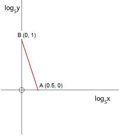
Gradient of BA:

\[ m = \frac{y_2 - y_1}{x_2 - x_1} \] \[ = \frac{0 - 1}{0.5 - 0} \] \[ = \frac{-1}{0.5} \] \[ = -2 \]

Line cuts the x‑axis at \((0,1)\), so:

\[ c = 1 \]

Graph is of the form \(Y = nX + c\), where \(Y = \log_5 y\), \(X = \log_5 x\), and \(c = \log_5 a\).

\[ \log y = n \log x + \log k \] Using base‑5 logs: \[ \log_{5} y = -2\,\log_{5} x + 1 \] Rewrite the straight‑line form back into an exponential: \[ \log_{5} y = \log_{5} x^{-2} + \log_{5} 5 \] Combine the logs: \[ \log_{5} y = \log_{5}\!\left(5\,x^{-2}\right) \] Remove the log: \[ y = 5\,x^{-2} \] And equivalently: \[ y = \frac{5}{x^{2}} \]

Books

Printed resources available at Amazon

Exponentials and Logarithms

Exponentials and Logarithms (Revision)

View on Amazon

These notes are suitable as a revision aid for anyone studying exponentials and logarithms.

Topics include:

Exponentials
Growth functions
Decay functions
Graphs: log scale on Y‑axis only
Graphs: log scale on both axes
Logarithms
Logarithmic equations
Graphs of exponential and log functions
Exponential functions
Logarithmic functions
Shifting log graphs

As an Amazon Associate I earn from qualifying purchases.