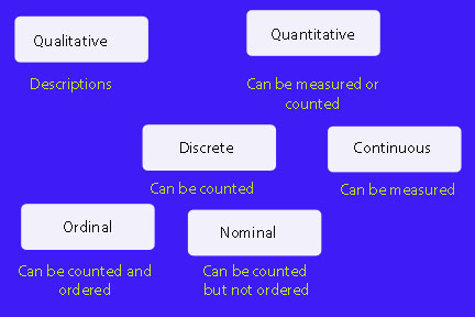
Maths Mutt HOME Statistics Hub


Statistical Terms

Definitions and vocabulary used in statistics


data

Qualitative Data

This is data which describes something categorical, e.g. "He is tall", "She has blue eyes".

Example

Favourite types of music:

  • Rock
  • Pop
  • Classical
  • Hip‑hop
  • Jazz

These categories describe types of music, not quantities, so they are qualitative data.

Quantitative Data

This is data which can be counted in numbers. It can be either continuous or discrete.

Example

Heights of students in a class (in centimetres):

  • 148 cm
  • 152 cm
  • 159 cm
  • 165 cm
  • 171 cm

These values are numerical and measurable, so they are quantitative data.

Continuous Data

This is data which can be measured.

Example

Temperatures recorded throughout a day (in °C):

  • 12.4°C
  • 13.0°C
  • 13.7°C
  • 14.1°C
  • 14.0°C

Temperature can take any value within a range and can be measured more precisely (e.g., to 1 decimal place, 2 decimal places, etc.), so it is continuous data.

Discrete Data

This is data which can be counted, e.g. number of legs, number of sunny days in June.

Discrete data is restricted to certain values, often whole numbers.

Discrete data can be ordinal or nominal.

Example

Number of goals scored in football matches:

  • 0 goals
  • 1 goal
  • 2 goals
  • 3 goals
  • 4 goals

You cannot score 2.5 goals — only whole numbers are possible — so this is discrete data.

Ordinal Data

(Ordered category data)

This is data which has categories which can be counted and ordered.

Example

Customer satisfaction ratings:

  • Very unhappy
  • Unhappy
  • Neutral
  • Happy
  • Very happy

These categories have a meaningful order, but the “distance” between them is not measurable.


Nominal Data

(Unordered category data)

This is data which can be counted but not ordered.

Example

Types of pets owned:

  • Dog
  • Cat
  • Rabbit
  • Fish
  • Hamster

These categories have no meaningful order — they are just labels — so this is nominal data.

The data is often displayed by a bar chart, pie chart or pictograph.

This is because a numerical relationship cannot be deduced for the information between the categories.


Population

A population is the complete set of persons, values or things for which data is being collected.

For example, all dogs in the UK would form the target population for a statistical analysis on dog food preferences.

Example

Suppose a vet wants to study the average weight of dogs in a town.

The population is:

  • All dogs living in that town

If the vet only weighs a smaller group of dogs, that smaller group becomes the sample, used to estimate the average weight of the whole population.

Census

A census collects data from the whole population.

Example

Suppose a town wants to know how many dogs live there.

A census would involve:

  • Counting every single dog in the town

This gives perfect information, but it takes far more time and effort than studying a smaller sample.

Sample

A sample collects data from a part of the population.

Example

Suppose the population is all dogs living in a town.

A sample might be:

  • 50 randomly chosen dogs from that town

These 50 dogs represent the whole population, allowing a vet or researcher to estimate things like the average weight or common health conditions without examining every single dog.

Batch Size

The batch size is the number of bits of data in the sample. It is given the letter n.

Example

batch size example

n = 15

Lower and Upper Extremes

The smallest data value in a batch is called the lower extreme and is given the symbol EL.

The largest data value in a batch is called the upper extreme and is given the symbol EU.

For the maths test scores data above, EL = 34% and EU = 86%.

Quartiles

Quartiles cut the data into quarters.

Q1 (also known as QL) is the lower quartile. This is the median of the lower half of data.

Q3 (also known as QU) is the upper quartile. This is the median of the upper half of data.

Each quartile represents 25%, so 50% of the data is represented between Q1 and Q3.

dfdf

Averages

There are three commonly used averages: mean, median and mode,

Example

Consider the data set:

4, 7, 7, 9, 10

  • Mean – add all the numbers and divide by how many there are.
    \( (4 + 7 + 7 + 9 + 10) ÷ 5 = 37 ÷ 5 = 7.4 \)
  • Median – the middle value when the numbers are in order.
    The middle number is 7.
  • Mode – the number that appears most often.
    The mode is 7 because it appears twice.

Each average tells us something slightly different about the data.

These are sometimes called measures of location.

Charts

Charts are used to display data visually.

Examples
  • Bar Chart – compares categories using bars of different lengths.
  • Pictogram – uses pictures or icons to represent quantities.
  • Pie Chart – shows how a whole is divided into parts.
  • Line Graph – shows how something changes over time.
  • Tally Chart – uses tally marks to count items quickly.

These charts are commonly used in school statistics and everyday data presentation.

Open Statistical Diagrams


Beagle Bytes
© Alexander Forrest