Maths Mutt HOME Statistics Hub


Calculated Statistics

Mean, median, mode, range, IQR, SD and more


Mean

The mean is the sum of the data divided by the number of bits of data.

This is also known as the arithmetical average.

\[ \text{Mean} \;=\; \frac{\text{Sum of all of the data}} {\text{Total number of bits of data}} \]

It is represented like this:

\[ \bar{X} = \frac{\sum X}{n} \]

\[ \bar{X} \text{ is called x bar and represents the mean} \] \[ \sum X \text{ is the sum of the data} \] \[ n \text{ is the number of bits of data (batch size)} \]

Example

Find the mean of the list:

2, 4, 6, 8, 12

\[ \text{Mean} = \frac{2 + 4 + 6 + 8 + 12}{5} \] \[ = \frac{32}{5} \] \[ = 6\frac{2}{5} \]

The formula can be re-arranged:

\[ \bar{X} = \frac{\sum X}{n} \]

\[ \bar{X}\, n \;=\; \sum X \]

\[ n \;=\; \frac{\displaystyle \sum X}{\bar{X}} \]

Example

Find the sum of the list of 8 numbers which has a mean of 18.

Sum = mean × n

= 18 × 8

= 144

Median

The middle value of an ordered batch of data is called the median.

Median = middle value of an ordered list.

If there are an odd number of bits of data, the median will be the value at \( \frac{1}{2}(n+1) \), where n is the batch size.

If there are an even number of bits of data, the median will be exactly halfway between the two values at \( \frac{1}{2}n \).

Example

Find the median of the list:

2, 6, 12, 8, 4

Here, n = 5

This is odd, so calculate \( \frac{1}{2}(n+1) \)

\( \frac{1}{2}(5+1) = 3 \)

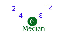
The median is the third number in the ordered list.

median odd example

This can be seen if the data is laid out like so:

median layout 1
Example

6, 8, 10, 2, 12, 4

Here, n = 6

This is even, so calculate \( \frac{1}{2}n \)

\( \frac{1}{2} \times 6 = 3 \)

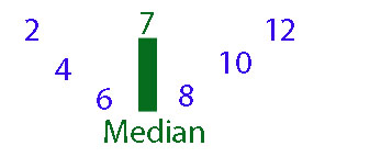
The median will be halfway between the 3rd and 4th numbers in the ordered list.

\[ \text{Median} = 2,\;4,\;6\;\uparrow\;8,\;10,\;12 \] \[ \text{Median is halfway between } 6 \text{ and } 8 \] \[ \text{Median} = \frac{6 + 8}{2} \] \[ \text{Median} = \frac{14}{2} \] \[ \text{Median} = 7 \]

This can be seen if the data is laid out like so:

median layout 2

Mode

The mode is the most recurring number in a list. Not all lists have a mode.

The Mode =The most occurring number.
Example
\[ \text{Find the Mode of the list:} \] \[ 2,\;4,\;6,\;8,\;12,\;12,\;15,\;4,\;2,\;6,\;8,\;7,\;7,\;9,\;12 \] \[ \text{Mode} = 12 \]
Example
\[ \text{Find the Mode of the list:} \] \[ 2,\;8,\;6,\;4,\;10,\;12,\;2,\;4,\;8,\;8,\;4 \] \[ \text{Mode} = 4 \text{ and } 8 \]

Range

The range is the difference between the highest and lowest numbers.

\[ \text{Range} = \text{Highest - Lowest} \]

Mid Range

The mid range is halfway between the highest and lowest values.

\[ \text{MidRange} = \frac{1}{2}\,( \text{Highest} + \text{Lowest} ) \]
Example

The list 2.5,4,33,6,7,9,8
Highest (H) = 33 , Lowest (L) = 2
\[ \text{Range} = 33 - 2 = 31 \]


\[ \text{MidRange} = \frac{1}{2}\,(\text{Highest} + \text{Lowest}) \] \[ = \frac{1}{2}\,(33 + 2) \] \[ = \frac{1}{2}\times 35 \] \[ = 17.5 \]

The five-figure summary

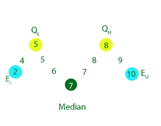
  • The highest Number   H ( also known as EU )
  • The lowest Number    L ( also known as EL )
  • The median, the number which halves the list  Q2 ( also known as M)
  • The upper quartile, the median of the upper half  Q3 ( also known as QU )
  • The lower quartile, the median of the lower half   Q1 ( also known as QL )
Example

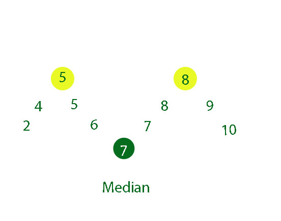
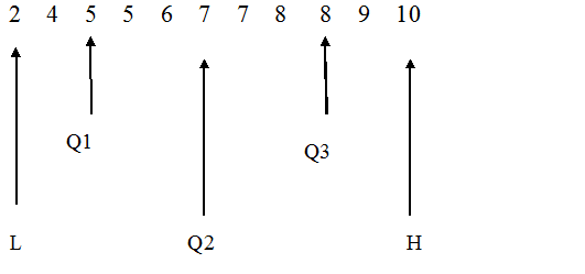
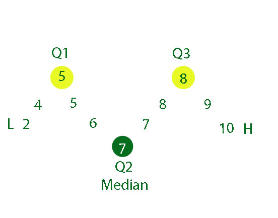
2   4   5   5   6   7   7   8   8  9    10 

jkk

n = 11

This is odd, so calculate 1/2( n+1)

1/2( n+1) = 1/2( 11+1) = 1/2 x 12 = 6

The median is the 6th position,  so Q2 = 7

There will be      (n-1) /2  numbers in each half.
So there will be 5 numbers in each half.
 The  lower quartile is the median of the lower half, so Q1 = 5
The upper quartile is the median of the upper half, so Q3 = 8

6


kl

or

bloy

5 -fig summary
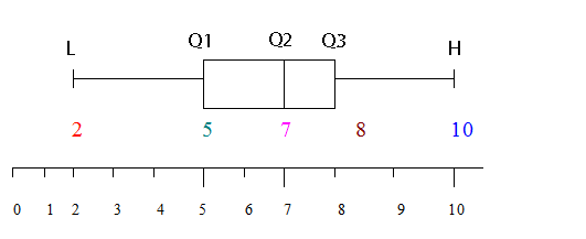
H = 10
L = 2
Q1 = 5
Q2 = 7
Q3 = 8

This information can be represented as a box plot :-

6 

Spread

spread

When comparing distributions, it is useful to know:

  • The central trend (mean, mode or median)
  • The spread (use range, interquartile range or semi‑interquartile range)

The spread in statistics — representing the variability or dispersion of a set of data values — measures how far the data points are from the centre or the average of the distribution. The further the spread, the less consistent the result.

The interquartile range is the range between the upper and lower quartiles.

Interquartile range = \( Q_3 - Q_1 \)

The Semi‑Interquartile Range (SIQR) is half of the interquartile range.

Semi‑Interquartile Range = \( \tfrac{1}{2}(Q_3 - Q_1) \)

Example

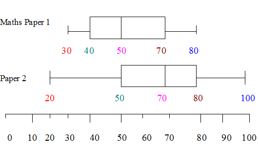
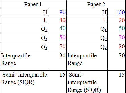
Compare the two sets of maths results.

table 7 table 8

Paper 2 has a better score overall, since more than three quarters of the candidates got a score of 50 or more, whereas only 50% of those sitting Paper 1 got between 50 and 80%.

Paper 2 has a larger spread of marks and a median of 70%, but both papers have the same interquartile range.

Skewness

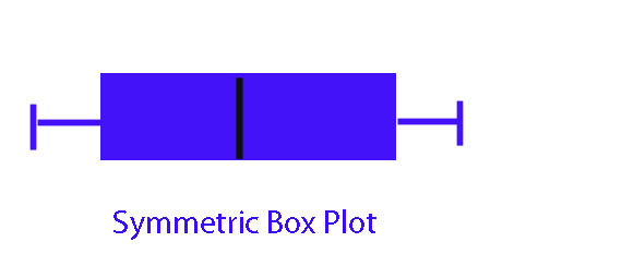
If the shape of the diagram is almost the same when a horizontal line is drawn across it, then the batch is symmetric.

symmetric diagram

The left-hand part is equal to the right-hand part,
or \(E_U - M = M - E_L\).

Otherwise, it is skew.

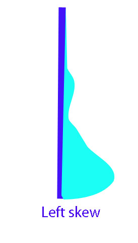
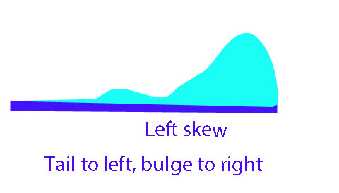
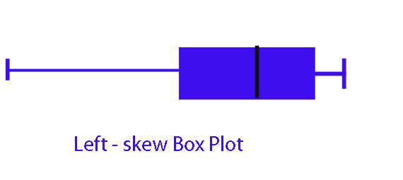
If the smaller values are further apart than the larger values, the batch is left-skew (the data bulges near the bottom).

left skew 1 left skew 2 left skew boxplot

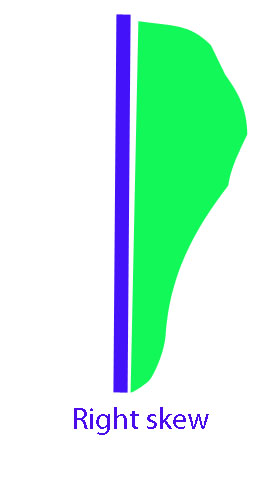
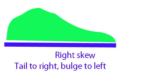
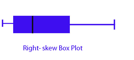
If the smaller values are closer together than the larger values, the batch is right-skew (the data bulges near the top).

The left-hand part is longer than the right-hand part,
or \(E_U - M < M - E_L\).

right skew 1 right skew 2 right skew boxplot

The right-hand part is longer than the left-hand part,
or \(E_U - M > M - E_L\).

Measure of Skewness based on Quartiles

\(Q_U\) = Upper Quartile (Q3)

\(Q_L\) = Lower Quartile (Q1)

\[ \frac{Q_U + Q_L - 2M}{dQ} \] \[ \frac{Q_U + Q_L - 2M}{\,Q_U - Q_L\,} \]

or

\[ \frac{Q_3 + Q_1 - 2Q_2}{\,Q_3 - Q_1\,} \]

If the result is positive, the data is right‑skewed.
If the result is negative, the data is left‑skewed.

Example

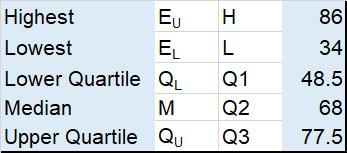
A 5‑figure summary of data gives:

five figure summary

\[ \frac{Q_U + Q_L - 2M}{\,Q_U - Q_L\,} \] \[ = \frac{77.5 + 48.5 - (2 \times 68)}{77.5 - 48.5} \] \[ = \frac{126 - 136}{29} \] \[ = \frac{-10}{29} \]

The value is negative, so the data is left‑skewed.

Standard Deviation

This is a measure of how much the data varies from the mean.

\[ s = \sqrt{\text{variance}} \]

Variance is the mean of the squares minus the square of the mean.

\[ \text{Variance} = \frac{\sum x^{2}}{n} \;-\; \left( \frac{\sum x}{n} \right)^{2} \]

A standard deviation of zero indicates that the data and the mean are effectively the same.

Two formulae are given by the SQA to calculate the standard deviation:

\[ s = \sqrt{ \frac{ \sum (x - \bar{x})^{2} }{ n - 1 } } \] and \[ s = \sqrt{ \frac{ \sum x^{2} \;-\; \frac{(\sum x)^{2}}{n} }{ n - 1 } } \]

Using the first equation

  • Find the mean by adding the data and dividing by n
  • Find the difference between the data and the mean (x̄)
  • Square these differences
  • Add up the total of the squared differences
  • Plug into the first equation given in the test paper

Using the second equation

  • Square the data to get \( x^2 \)
  • Find totals \( \Sigma x \) and \( \Sigma x^2 \)
  • Square the total \( \Sigma x \) and divide by n
  • Plug into the second equation given in the test paper
Example

Calculate the standard deviation of the numbers:
101, 105, 133, 142, 185, 186

First Equation
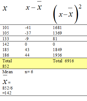
sd example 1
  • Find the mean
  • Find the differences from the mean
  • Square the differences
  • Add the squared differences
  • Substitute into the formula
\[ s = \sqrt{ \frac{ \sum (x - \bar{x})^{2} }{ n - 1 } } \] \[ = \sqrt{ \frac{ 6916 }{ 6 - 1 } } \] \[ = \sqrt{ \frac{6916}{5} } \] \[ = 37.1914 \]

Using equation 2
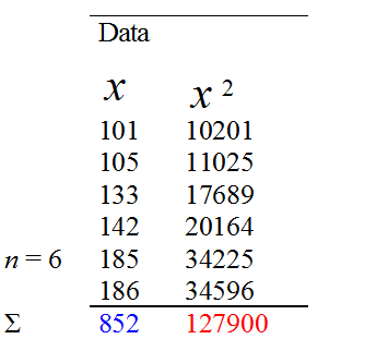
sd example 2
  • Square the data
  • Find totals \( \Sigma x \) and \( \Sigma x^2 \)
  • Square \( \Sigma x \) and divide by n
  • Substitute into the formula
\[ s = \sqrt{ \frac{ \sum x^{2} \;-\; \frac{(\sum x)^{2}}{n} }{ n - 1 } } \] \[ s = \sqrt{ \frac{ \color{red}{127900} \;-\; \frac{\color{blue}{852}^{2}}{6} }{ 6 - 1 } } \] \[ s = \sqrt{ \frac{ 127900 \;-\; \frac{725904}{6} }{ 5 } } \] \[ s = \sqrt{ \frac{ 127900 - 120984 }{ 5 } } \] \[ s = \sqrt{ \frac{6916}{5} } \] \[ s = \sqrt{1383.2} \] \[ s = 37.1914 \]

Changing all of the numbers by the same amount does not affect the standard deviation.

Example

The standard deviation of:

101, 105, 133, 142, 185, 186

is the same as the standard deviation of:

1, 5, 33, 42, 85, 86

and

4, 8, 36, 45, 88, 89

Interactive - Standard Deviation

Frequency Tables

These are a useful way of collating raw data, to quickly see the mode, find the median, and calculate the mean.

Example

A manufacturer claims that each packet of Shazbo contains 20 sweets on average.

When 30 packets of Shazbo are examined, the results are as follows:

No. of sweets per packet:

18 17 22 19 20 20 21 19 18 20

21 19 21 19 20 20 20 17 19 21

22 18 17 16 20 20 20 21 21 20

Is the manufacturer correct?

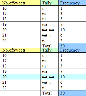
Construct a frequency table of the data.

frequency table

The table shows that the mode of the sample is 20 sweets, which has a frequency of 10.

The median value lies halfway between the 15th and 16th values.

The frequency column shows that the first 12 values have between 16 and 19 sweets. The 15th and 16th values have 20 sweets.

The median is therefore 20 sweets.

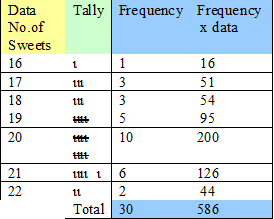
To calculate the mean, we need to add another column and multiply the frequency by the number of sweets.

mean table 1 \[ \text{mean} = \frac{\text{total number of sweets}}{\text{number of packets}} \] \[ = \frac{586}{30} \] \[ = 19 \frac{16}{30} \] \[ = 19 \frac{8}{15} \] \[ = 19.533333 \]

The mean is 19½ sweets, which could be rounded to 20 sweets.

The manufacturer is correct!

Grouped Frequency Tables and Midpoint Class Intervals

These are used when the data is sorted into intervals.

Example

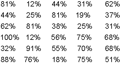
The scores for an S4 homework are shown below as percentages.

grouped data

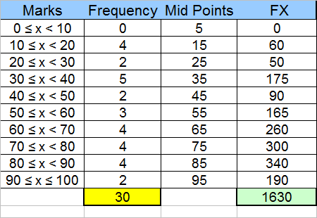
Firstly, the data is sorted into equal intervals.

  • The midpoint is found by adding the end intervals and halving the result
  • The frequency is then multiplied by the midpoint
grouped frequency table

The modal interval is 30 to 39.

The mean is 1630 / 30 = 54.3333

The median is halfway between the 15th and 16th items. This is found by adding the frequencies and occurs in the interval 51 to 60.

Relative Frequency

The relative frequency is a measure of the fraction of the data. It can be used to predict amounts.

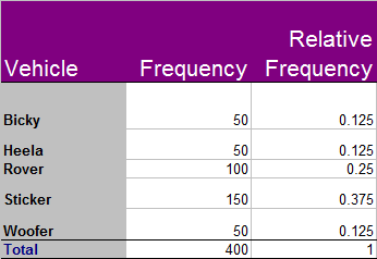
To find the relative frequency, divide the frequency for the particular item by the total frequency of the data.

The total relative frequency must always be 1.

Example

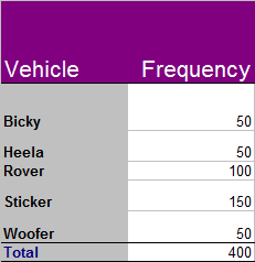
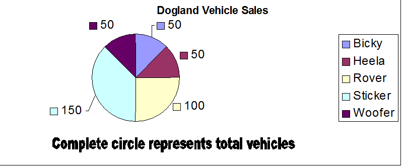
The following vehicles were sold in Dogland:

vehicle table

How many Woofers are expected to be sold per 1000 vehicles?

woofer calculation

Woofers account for 12.5% of the vehicle sales, so for every 1,000 vehicles sold, 125 of them would be expected to be a Woofer.

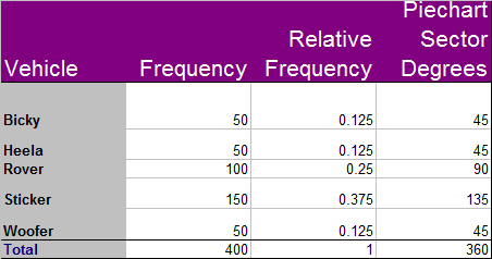
To display the data as a pie chart, calculate the fraction of 360°:

pie chart calculation pie chart

Books

Printed resources available at Amazon

Mean, Median, Mode and Range

Mean, Median, Mode and Range (Drill Questions)

View on Amazon

This book contains 2,000 drill questions — each requiring the mean, median, mode and range to be calculated for a data set.

Basic Statistics & Probability

Basic Statistics & Probability (Revision)

View on Amazon

Revision notes for basic statistics and probability, suitable for BGE Information Handling, National 4, National 5, and Higher.

Topics include:

  • Basic statistical terms
  • Mean, Median, Mode, Range
  • Five‑figure summary and SIQR
  • Stem & Leaf, Dot Plot, Box Plot
  • Standard Deviation
  • Frequency Tables, Cumulative Frequency
  • Grouped Frequency midpoints
  • Relative frequency
  • Line of Best Fit
  • Probability
  • Mutually exclusive events, addition & multiplication laws
  • Tree diagrams

As an Amazon Associate I earn from qualifying purchases.


Beagle Bytes
© Alexander Forrest