Physical quantities fall into two categories:
Scalar or Vector
Scalars
A scalar quantity is defined by its
magnitude and units.
A few scalars:
- Distance
- Speed
- Time
- Temperature
- Energy
- Work
- Power
- Mass
- Volume
- Area
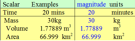
A speed of 60 mph is a scalar quantity.
Vectors
A vector quantity is defined by its
magnitude, units, and
direction.
A few vectors:
- Displacement
- Velocity
- Acceleration
- Force
- Weight
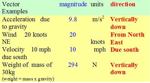
Speed is not a vector, since it doesn’t have a direction.
Velocity is a vector, so must have a direction.
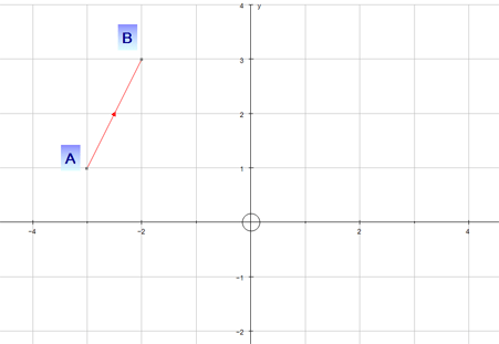
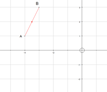
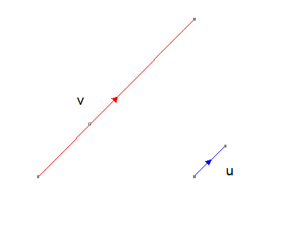
A vector can be drawn as a line, with length representing magnitude and an arrow showing direction.
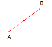
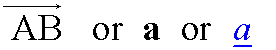
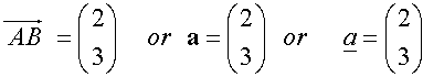
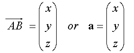
Vector AB is written as:

The vectors below are shown in component form:
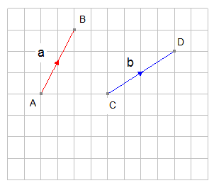
Vector AB is written as:
B is 2 units right and 3 units up from A.
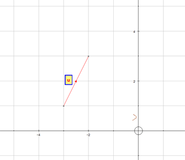
The components are written as a column vector:
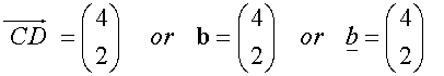
Likewise:
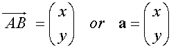
When the coordinates of endpoints are not known:
Or in 3‑D:
When the coordinates of endpoints are known:
Or in 3‑D:
Example
\[
\text{Find the components of the vector joining the points }
S(6,8)\ \text{and}\ B(-5,6)
\]
\[
\overrightarrow{SB}
=
\begin{pmatrix}
-5 \\[4pt]
6
\end{pmatrix}
-
\begin{pmatrix}
6 \\[4pt]
8
\end{pmatrix}
=
\begin{pmatrix}
-11 \\[4pt]
-2
\end{pmatrix}
\]
Example
\[
\text{The vector }\mathbf{d}
=
\begin{pmatrix}
5 \\[4pt]
2
\end{pmatrix}
\text{ is applied to the point }H(3,-1)\text{ to make }\overrightarrow{HP}.
\text{ Find the co-ordinates of} P\]
\[
\mathbf{d}
=
\begin{pmatrix}
5 \\[4pt]
2
\end{pmatrix}
=
\overrightarrow{HP}
=
\begin{pmatrix}
x_P \\[4pt]
y_P
\end{pmatrix}
-
\begin{pmatrix}
x_H \\[4pt]
y_H
\end{pmatrix}
\]
\[
\text{with }H(3,-1)\text{, so}
\qquad
\begin{pmatrix}
5 \\[4pt]
2
\end{pmatrix}
=
\begin{pmatrix}
x_P - 3 \\[4pt]
y_P + 1
\end{pmatrix}.
\]
\[
\text{so}
\]
\[
\begin{pmatrix}
5 \\[4pt]
2
\end{pmatrix}
=
\begin{pmatrix}
x_P \\[4pt]
y_P
\end{pmatrix}
-
\begin{pmatrix}
3 \\[4pt]
-1
\end{pmatrix}
\]
\[
5 = x_P - 3
\qquad\qquad
2 = y_P + 1
\]
\[
\Rightarrow\quad
x_P = 8
\qquad\qquad
\Rightarrow\quad
y_P = 1
\]
\[
P(8,\,1)
\]
Each of these lines represents the vector:

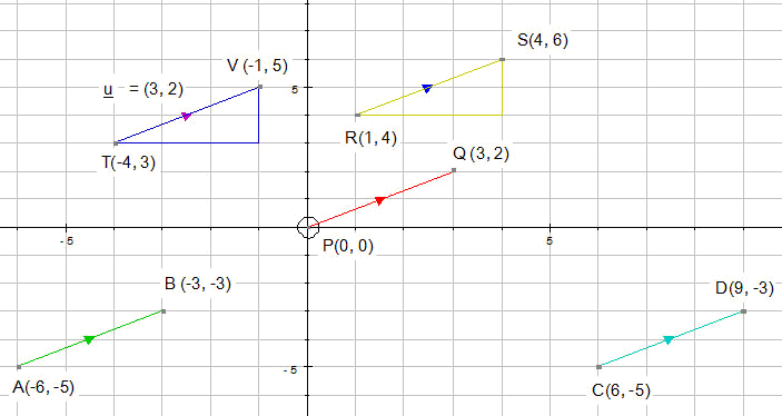
\[
\overrightarrow{TV}
=
\overrightarrow{RS}
=
\overrightarrow{PQ}
=
\overrightarrow{AB}
=
\overrightarrow{CD}
=
\mathbf{u}
\]
\[
\text{So }
TV = RS = PQ = AB = CD
\quad\text{(i.e. all of equal length)}
\]
\[
\text{and }
TV \parallel RS \parallel PQ \parallel AB \parallel CD
\quad\text{(i.e. all parallel)}
\]
Direction is important
\[
\overrightarrow{AB}
=
\begin{pmatrix}
3 \\[4pt]
2
\end{pmatrix}
\qquad\qquad
\overrightarrow{BA}
=
\begin{pmatrix}
-3 \\[4pt]
-2
\end{pmatrix}
\]
\[
\overrightarrow{AB} \ne \overrightarrow{BA}
\qquad\qquad
\overrightarrow{AB} = -\,\overrightarrow{BA}
\]
\[
\text{If }\mathbf{u} =
\begin{pmatrix}
a \\[4pt]
b
\end{pmatrix}
\quad\text{then}\quad
-\mathbf{u} =
\begin{pmatrix}
-\,a \\[4pt]
-\,b
\end{pmatrix}
\]
A vector is the hypotenuse of the right‑angled triangle formed by its components.
The magnitude is found using Pythagoras’ Theorem.
\[
\mathbf{v}
=
\begin{pmatrix}
x \\[4pt]
y
\end{pmatrix}
\quad\text{has magnitude}\quad
|\mathbf{v}|
=
\sqrt{x^{2} + y^{2}}
\]
\[
\mathbf{v}
=
\begin{pmatrix}
x \\[4pt]
y \\[4pt]
z
\end{pmatrix}
\quad\text{has magnitude}\quad
|\mathbf{v}|
=
\sqrt{x^{2} + y^{2} + z^{2}}
\]
The magnitude is always positive.
Examples
\[
\mathbf{c}
=
\begin{pmatrix}
3 \\[4pt]
4
\end{pmatrix}
\]
\[
|\mathbf{c}|
=
\sqrt{3^{2} + 4^{2}}
\]
\[
= \sqrt{9 + 16}
\]
\[
= 5
\]
\[
\overrightarrow{FG}
=
\begin{pmatrix}
3 \\[4pt]
5
\end{pmatrix}
\]
\[
\left|\overrightarrow{FG}\right|
=
\sqrt{3^{2} + 5^{2}}
\]
\[
= \sqrt{9 + 25}
\]
\[
= 5.83095
\]
\[
\left|\overrightarrow{FG}\right|
= 5.83095
\]
\[
\mathbf{s}
=
\begin{pmatrix}
-4 \\[4pt]
8 \\[4pt]
-1
\end{pmatrix}
\]
\[
|\mathbf{s}|
=
\sqrt{(-4)^{2} + 8^{2} + (-1)^{2}}
\]
\[
= \sqrt{16 + 64 + 1}
\]
\[
= \sqrt{81}
\]
\[
= 9
\]
Example
Three points P(3,4,−1), Q(9,8,11), R(−9,−2,3). Show triangle PQR is isosceles.
\[
\overrightarrow{PQ}
=
\begin{pmatrix}
9 - 3 \\[4pt]
8 - 4 \\[4pt]
11 - (-1)
\end{pmatrix}
\]
\[
\text{so}\quad
\overrightarrow{PQ}
=
\begin{pmatrix}
6 \\[4pt]
4 \\[4pt]
12
\end{pmatrix}
\]
\[
\overrightarrow{QR}
=
\begin{pmatrix}
(-9) - 9 \\[4pt]
(-2) - 8 \\[4pt]
3 - 11
\end{pmatrix}
\]
\[
\text{so}\quad
\overrightarrow{QR}
=
\begin{pmatrix}
-18 \\[4pt]
-10 \\[4pt]
-8
\end{pmatrix}
\]
\[
\overrightarrow{PR}
=
\begin{pmatrix}
(-9) - 3 \\[4pt]
(-2) - 4 \\[4pt]
3 - (-1)
\end{pmatrix}
\]
\[
\text{so}\quad
\overrightarrow{PR}
=
\begin{pmatrix}
-12 \\[4pt]
-6 \\[4pt]
4
\end{pmatrix}
\]
\[
\left|\overrightarrow{PQ}\right|
=
\sqrt{6^{2} + 4^{2} + 12^{2}}
\]
\[
= \sqrt{36 + 16 + 144}
\]
\[
= \sqrt{196}
\]
\[
= 14
\]
\[
\left|\overrightarrow{PQ}\right| = 14
\]
\[
\left|\overrightarrow{QR}\right|
=
\sqrt{(-18)^{2} + (-10)^{2} + (-8)^{2}}
\]
\[
= \sqrt{324 + 100 + 64}
\]
\[
= \sqrt{488}
\]
\[
= 22.0907
\]
\[
\left|\overrightarrow{QR}\right| = 22.1
\]
\[
\left|\overrightarrow{PR}\right|
=
\sqrt{(-12)^{2} + (-6)^{2} + 4^{2}}
\]
\[
= \sqrt{144 + 36 + 16}
\]
\[
= \sqrt{196}
\]
\[
\left|\overrightarrow{PR}\right| = 14
\]
\[
\text{Since }\;
\left|\overrightarrow{PR}\right|
=
\left|\overrightarrow{PQ}\right|
= 14,
\quad
\triangle PQR \text{ is isosceles.}
\]
Interactive – Vector Magnitudes
Vectors are added nose‑to‑tail.
\[
\text{For vectors }\mathbf{u}\text{ and }\mathbf{v}
\]
\[
\text{if }\;
\mathbf{u}
=
\begin{pmatrix}
a \\[4pt]
b
\end{pmatrix}
\qquad\text{and}\qquad
\mathbf{v}
=
\begin{pmatrix}
c \\[4pt]
d
\end{pmatrix}
\]
\[
\text{then }\;
\mathbf{u} + \mathbf{v}
=
\begin{pmatrix}
a + c \\[4pt]
b + d
\end{pmatrix}
\]
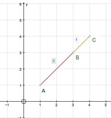
Example
\[
\overrightarrow{AB}
=
\begin{pmatrix}
1 \\[4pt]
2
\end{pmatrix}
\qquad
\overrightarrow{BC}
=
\begin{pmatrix}
5 \\[4pt]
-3
\end{pmatrix}
\qquad
\overrightarrow{AC}
=
\begin{pmatrix}
6 \\[4pt]
-1
\end{pmatrix}
\]
\[
\overrightarrow{AB}
+
\overrightarrow{BC}
=
\begin{pmatrix}
1 \\[4pt]
2
\end{pmatrix}
+
\begin{pmatrix}
5 \\[4pt]
-3
\end{pmatrix}
=
\begin{pmatrix}
6 \\[4pt]
-1
\end{pmatrix}
=
\overrightarrow{AC}
\]
Example
\[
\mathbf{s}
=
\begin{pmatrix}
3 \\[4pt]
2
\end{pmatrix}
\qquad
\mathbf{r}
=
\begin{pmatrix}
5 \\[4pt]
-6
\end{pmatrix}
\qquad
\mathbf{g}
=
\begin{pmatrix}
10 \\[4pt]
-1
\end{pmatrix}
\]
\[
\text{Find the components of:}
\]
\[
\text{a) }\mathbf{s} + \mathbf{r}
\qquad
\text{b) }\mathbf{s} + \mathbf{g}
\qquad
\text{c) }\mathbf{s} + \mathbf{g} + \mathbf{r}
\qquad
\text{d) }\mathbf{s} + \mathbf{r} + \mathbf{g}
\]
\[
\text{a) }\mathbf{s} + \mathbf{r}
=
\begin{pmatrix}
3 \\[4pt]
2
\end{pmatrix}
+
\begin{pmatrix}
5 \\[4pt]
-6
\end{pmatrix}
=
\begin{pmatrix}
8 \\[4pt]
-4
\end{pmatrix}
\]
\[
\text{b) }\mathbf{s} + \mathbf{g}
=
\begin{pmatrix}
3 \\[4pt]
2
\end{pmatrix}
+
\begin{pmatrix}
10 \\[4pt]
-1
\end{pmatrix}
=
\begin{pmatrix}
13 \\[4pt]
1
\end{pmatrix}
\]
\[
\text{c) }\mathbf{s} + \mathbf{g} + \mathbf{r}
=
\begin{pmatrix}
3 \\[4pt]
2
\end{pmatrix}
+
\begin{pmatrix}
10 \\[4pt]
-1
\end{pmatrix}
+
\begin{pmatrix}
5 \\[4pt]
-6
\end{pmatrix}
=
\begin{pmatrix}
18 \\[4pt]
-5
\end{pmatrix}
\]
\[
\text{d) }\mathbf{s} + \mathbf{r} + \mathbf{g}
=
\begin{pmatrix}
3 \\[4pt]
2
\end{pmatrix}
+
\begin{pmatrix}
5 \\[4pt]
-6
\end{pmatrix}
+
\begin{pmatrix}
10 \\[4pt]
-1
\end{pmatrix}
=
\begin{pmatrix}
18 \\[4pt]
-5
\end{pmatrix}
\]
\[
\text{For vectors }\mathbf{u}\text{ and }\mathbf{v}
\]
\[
\text{if }\;
\mathbf{u}
=
\begin{pmatrix}
a \\[4pt]
b
\end{pmatrix}
\qquad\text{and}\qquad
\mathbf{v}
=
\begin{pmatrix}
c \\[4pt]
d
\end{pmatrix}
\]
\[
\text{then}
\]
\[
\mathbf{u} - \mathbf{v}
=
\mathbf{u} + (-\mathbf{v})
\]
\[
=
\begin{pmatrix}
a \\[4pt]
b
\end{pmatrix}
+
\begin{pmatrix}
-\,c \\[4pt]
-\,d
\end{pmatrix}
\]
\[
=
\begin{pmatrix}
a - c \\[4pt]
b - d
\end{pmatrix}
\]
Example
\[
\mathbf{u}
=
\begin{pmatrix}
1 \\[4pt]
2
\end{pmatrix},
\qquad
\mathbf{v}
=
\begin{pmatrix}
3 \\[4pt]
2
\end{pmatrix}
\]
\[
\mathbf{u} - \mathbf{v}
=
\begin{pmatrix}
1 \\[4pt]
2
\end{pmatrix}
+
\begin{pmatrix}
-3 \\[4pt]
-2
\end{pmatrix}
=
\begin{pmatrix}
-2 \\[4pt]
0
\end{pmatrix}
\]
The shape below is a square‑based pyramid.
\[
\overrightarrow{AB}
=
\mathbf{u}
\]
\[
\overrightarrow{CB}
=
\mathbf{V}
\]
\[
\overrightarrow{EB}
=
\mathbf{w}
\]
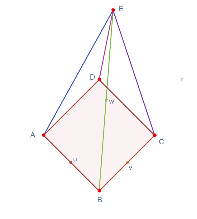
To go from A to C, go AB followed by BC.
This is the same as u - v
\[
\overrightarrow{AC}
=
\mathbf{u} - \mathbf{v}
\]
\[
\overrightarrow{AE}
=
\mathbf{u} - \mathbf{w}
\]
\[
\overrightarrow{ED}
=
\mathbf{w} - \mathbf{v} - \mathbf{u}
\]
The zero vector is the vector that has no length and no direction. In component form it’s written as
\(\mathbf{0}
=
\begin{pmatrix}
0 \\[4pt]
0
\end{pmatrix}
\) or
\(
\mathbf{0}
=
\begin{pmatrix}
0 \\[4pt]
0 \\[4pt]
0
\end{pmatrix}
\)
It acts as the identity element for vector addition: adding the zero vector doesn’t change anything.
It represents “no movement” — staying exactly where you are.
Travelling from A to B and back gives zero displacement, but the distance travelled is the sum of magnitudes.
Example
\[
\mathbf{u} = \overrightarrow{AB}
=
\begin{pmatrix}
1 \\[4pt]
2
\end{pmatrix}
\qquad
\mathbf{v} = \overrightarrow{BC}
=
\begin{pmatrix}
4 \\[4pt]
-2
\end{pmatrix}
\]
\[
\mathbf{w} = \overrightarrow{CD}
=
\begin{pmatrix}
-6 \\[4pt]
-3
\end{pmatrix}
\qquad
\mathbf{x} = \overrightarrow{DA}
=
\begin{pmatrix}
1 \\[4pt]
3
\end{pmatrix}
\]
\[
\text{then }
\mathbf{u} + \mathbf{v} + \mathbf{w} + \mathbf{x}
=
\begin{pmatrix}
1 + 4 + (-6) + 1 \\[6pt]
2 + (-2) + (-3) + 3
\end{pmatrix}
=
\begin{pmatrix}
0 \\[4pt]
0
\end{pmatrix}
\]
\[
\text{This is the zero vector } \mathbf{0}.
\]
For any vector v, there is a parallel unit vector of magnitude 1.
Example
\[
\mathbf{v}
=
\begin{pmatrix}
8 \\[4pt]
6
\end{pmatrix}
\]
\[
\left|\mathbf{v}\right|
=
\sqrt{8^{2} + 6^{2}}
\]
\[
= \sqrt{100}
\]
\[
= 10
\]
\[
\mathbf{u}
=
\frac{1}{10}\,\mathbf{v}
\]
\[
=
\frac{1}{10}
\begin{pmatrix}
8 \\[4pt]
6
\end{pmatrix}
\]
\[
=
\begin{pmatrix}
\frac{8}{10} \\[6pt]
\frac{6}{10}
\end{pmatrix}
\]
\[
=
\begin{pmatrix}
\frac{4}{5} \\[6pt]
\frac{3}{5}
\end{pmatrix}
\]
A position vector is given relative to the origin O.
Example
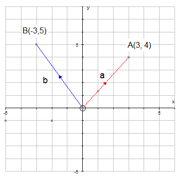
\[
\overrightarrow{OA}
\text{ is written }
\mathbf{a},
\qquad
\mathbf{a}
=
\begin{pmatrix}
3 \\[4pt]
4
\end{pmatrix}
\]
\[
\overrightarrow{OB}
\text{ is written }
\mathbf{b},
\qquad
\mathbf{b}
=
\begin{pmatrix}
-3 \\[4pt]
5
\end{pmatrix}
\]
\[
\overrightarrow{AB}
=
\mathbf{b} - \mathbf{a}
\]
\[
=
\begin{pmatrix}
-3 \\[4pt]
5
\end{pmatrix}
-
\begin{pmatrix}
3 \\[4pt]
4
\end{pmatrix}
\]
\[
=
\begin{pmatrix}
-6 \\[4pt]
1
\end{pmatrix}
\]
\[
\overrightarrow{AB}
=
\mathbf{b} - \mathbf{a}
\]
\[
\text{where }\mathbf{a}\text{ and }\mathbf{b}\text{ are the position vectors of A and B.}
\]
A vector may be described in terms of unit vectors i, j and k:
\[
\mathbf{i}
=
\begin{pmatrix}
1 \\[4pt]
0 \\[4pt]
0
\end{pmatrix}
\qquad
\mathbf{j}
=
\begin{pmatrix}
0 \\[4pt]
1 \\[4pt]
0
\end{pmatrix}
\qquad
\mathbf{k}
=
\begin{pmatrix}
0 \\[4pt]
0 \\[4pt]
1
\end{pmatrix}
\]
Example
\[
\begin{pmatrix}
4 \\[4pt]
2 \\[4pt]
-5
\end{pmatrix}
=
4
\begin{pmatrix}
1 \\[4pt]
0 \\[4pt]
0
\end{pmatrix}
+
2
\begin{pmatrix}
0 \\[4pt]
1 \\[4pt]
0
\end{pmatrix}
-
5
\begin{pmatrix}
0 \\[4pt]
0 \\[4pt]
1
\end{pmatrix}
\]
\[
= 4\mathbf{i} + 2\mathbf{j} - 5\mathbf{k}
\]
The position vector of (x, y, z) is:
\[
\mathbf{r}
=
x\mathbf{i}
+
y\mathbf{j}
+
z\mathbf{k}
\]
Multiplication of a vector by a Scalar
\[
\text{If }\mathbf{u}
=
\begin{pmatrix}
x \\[4pt]
y
\end{pmatrix}
\text{ then }
k\mathbf{u}
=
\begin{pmatrix}
kx \\[4pt]
ky
\end{pmatrix}
\]
Example
\[
\text{If }\mathbf{u}
=
\begin{pmatrix}
1 \\[4pt]
3
\end{pmatrix}
\]
\[
\text{then }2\mathbf{u}
=
\begin{pmatrix}
2 \times 1 \\[4pt]
2 \times 3
\end{pmatrix}
=
\begin{pmatrix}
2 \\[4pt]
6
\end{pmatrix}
\]
\[
\text{and }\tfrac12\mathbf{u}
=
\begin{pmatrix}
\frac12 \times 1 \\[4pt]
\frac12 \times 3
\end{pmatrix}
=
\begin{pmatrix}
\frac12 \\[6pt]
\frac32
\end{pmatrix}
\]
\[
\text{If }\mathbf{u}
=
\begin{pmatrix}
x \\[4pt]
y
\end{pmatrix}
\text{ then }
k\mathbf{u}
=
\begin{pmatrix}
kx \\[4pt]
ky
\end{pmatrix}
\text{ and }\mathbf{u}\text{ is parallel to }k\mathbf{u}.
\]
\[
\text{Conversely, if }\mathbf{u}\text{ is parallel to }k\mathbf{u}
\text{ then }\mathbf{u} = k\mathbf{u}.
\]
\[
\text{Collinear points lie on a straight line.}
\]
\[
\text{If }\overrightarrow{AB} = k\,\overrightarrow{BC}
\text{ (where \(k\) is a scalar), then }
\overrightarrow{AB} \parallel \overrightarrow{BC}.
\]
\[
\text{If B is a point common to both AB and BC, then A, B, C are collinear.}
\]
Example
Prove A(1,1), B(3,3), C(4,4) are collinear and find the ratio in which B divides AC.
\[
\overrightarrow{AB}
=
\begin{pmatrix}
3 \\[4pt]
3
\end{pmatrix}
-
\begin{pmatrix}
1 \\[4pt]
1
\end{pmatrix}
=
\begin{pmatrix}
2 \\[4pt]
2
\end{pmatrix}
\]
\[
\overrightarrow{BC}
=
\begin{pmatrix}
4 \\[4pt]
4
\end{pmatrix}
-
\begin{pmatrix}
3 \\[4pt]
3
\end{pmatrix}
=
\begin{pmatrix}
1 \\[4pt]
1
\end{pmatrix}
\]
\[
\overrightarrow{AB}
=
\begin{pmatrix}
2 \\[4pt]
2
\end{pmatrix}
=
2
\begin{pmatrix}
1 \\[4pt]
1
\end{pmatrix}
=
2\,\overrightarrow{BC}
\]
\[
\text{Therefore, AB is parallel to BC.}
\]
\[
\text{Since B is common to both AB and BC, A, B and C are collinear.}
\]
Ratio in which B divides AC:
\[
\overrightarrow{AB}
=
2\,\overrightarrow{BC}
\]
\[
1\,\overrightarrow{AB}
=
2\,\overrightarrow{BC}
\]
\[
\frac12\,\overrightarrow{AB}
=
\overrightarrow{BC}
\]
\[
\text{(cannot divide vectors)}
\]
\[
\Rightarrow\;
\frac{\overrightarrow{BC}}{\overrightarrow{AB}}
=
\frac12
\]
AB : BC = 2 : 1
B divides AC internally in the ratio 2 : 1.
Example
Given A(1,1), B(6,6), C(4,4) are collinear, find the ratio in which B divides AC.
\[
\overrightarrow{AB}
=
\begin{pmatrix}
6 \\[4pt]
6
\end{pmatrix}
-
\begin{pmatrix}
1 \\[4pt]
1
\end{pmatrix}
=
\begin{pmatrix}
5 \\[4pt]
5
\end{pmatrix}
\]
\[
\overrightarrow{BC}
=
\begin{pmatrix}
4 \\[4pt]
4
\end{pmatrix}
-
\begin{pmatrix}
6 \\[4pt]
6
\end{pmatrix}
=
\begin{pmatrix}
-2 \\[4pt]
-2
\end{pmatrix}
\]
\[
\overrightarrow{AB}
=
\begin{pmatrix}
5 \\[4pt]
5
\end{pmatrix}
=
\frac{5}{-2}
\begin{pmatrix}
-2 \\[4pt]
-2
\end{pmatrix}
=
\frac{5}{-2}\,\overrightarrow{BC}
\]
\[
\overrightarrow{AB}
=
\frac{5}{-2}\,\overrightarrow{BC}
\]
\[
-2\,\overrightarrow{AB}
=
5\,\overrightarrow{BC}
\]
\[
\frac{-2}{5}\,\overrightarrow{AB}
=
\overrightarrow{BC}
\]
\[
\text{(cannot divide vectors)}
\]
\[
\Rightarrow\;
\frac{\overrightarrow{BC}}{\overrightarrow{AB}}
=
\frac{-2}{5}
\]
AB : BC = 5 : −2
B divides AC externally in the ratio 5 : −2.
\[
\mathbf{p}
=
\frac{n}{m+n}\,\mathbf{a}
+
\frac{m}{m+n}\,\mathbf{b}
\]
\[
\text{Where }\mathbf{p}\text{ is the position vector of the point }P
\]
\[
\text{that divides }AB\text{ in the ratio }m:n.
\]
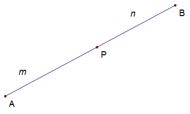
Why does this work?
Take the points A and B and join them together with a straight line. Now let P be a point which cuts line AB in the ratio 1:2
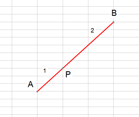
so that the length of AP is one half of the length PB
The points A and P can be represented by their position vectors.
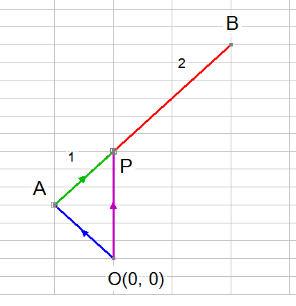
By vector addition,
\[
\overrightarrow{OP}
=
\overrightarrow{OA}
+
\overrightarrow{AP}
\]
Writing position vectors as vectors gives
\(\overrightarrow{OP}
=
\mathbf{p}
\) and
\(
\overrightarrow{OA}
=
\mathbf{a}
\)
Since P splits AB in the ratio is 1:2
\[
\overrightarrow{AP}
=
\frac{1}{3}\,\overrightarrow{AB}
\]
and
\[
\overrightarrow{AB}
=
\mathbf{b} - \mathbf{a}
\]
So
\[
\overrightarrow{OP}
=
\overrightarrow{OA}
+
\overrightarrow{AP}
\]
\[
\mathbf{p}
=
\mathbf{a}
+
\frac{1}{3}\,\overrightarrow{AB}
\]
\[
=
\mathbf{a}
+
\frac{1}{3}\,(\mathbf{b} - \mathbf{a})
\]
multiplying out the brackets
\[
\mathbf{p}
=
\mathbf{a}
+
\frac{1}{3}(\mathbf{b} - \mathbf{a})
\]
\[
=
\mathbf{a}
+
\frac{1}{3}\mathbf{b}
-
\frac{1}{3}\mathbf{a}
\]
\[
=
\frac{2}{3}\mathbf{a}
+
\frac{1}{3}\mathbf{b}
\]
Notice that the numerator of a is 2 , which is the value of length n, and that of b is 1, which is the value of length m.
Also notice that the denominator of both is m+n.
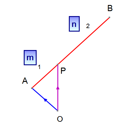
So
\[
\mathbf{p}
=
\frac{n}{m+n}\,\mathbf{a}
+
\frac{m}{m+n}\,\mathbf{b}
\]
Or , if preferred , written b first
\[ \mathbf{p} = \frac{m}{m+n}\,\mathbf{b} + \frac{n}{m+n}\,\mathbf{a} \]
Example
A and B have co-ordinates (6,7) and (16,22) respectively.
Find the co-ordinates of the point P if AP:PB = 2:3.
Find the lengths of AB, AP and PB and check that the stated ratios are correct.
\[
\mathbf{p}
=
\frac{n}{m+n}\,\mathbf{a}
+
\frac{m}{m+n}\,\mathbf{b}
\]
\[
=
\frac{3}{5}\,\mathbf{a}
+
\frac{2}{5}\,\mathbf{b}
\]
\[
=
\frac{1}{5}\,(3\mathbf{a} + 2\mathbf{b})
\]
\[
=
\frac{1}{5}
\left(
3
\begin{pmatrix}
6 \\[4pt]
7
\end{pmatrix}
+
2
\begin{pmatrix}
16 \\[4pt]
22
\end{pmatrix}
\right)
\]
\[
=
\frac{1}{5}
\left(
\begin{pmatrix}
18 \\[4pt]
21
\end{pmatrix}
+
\begin{pmatrix}
32 \\[4pt]
44
\end{pmatrix}
\right)
\]
\[
=
\frac{1}{5}
\begin{pmatrix}
50 \\[4pt]
65
\end{pmatrix}
\]
\[
=
\begin{pmatrix}
10 \\[4pt]
13
\end{pmatrix}
\]
\[
\text{P has the coordinates }(10,13).
\]
Alternatively:
\[
3\,\overrightarrow{AP}
=
2\,\overrightarrow{PB}
\]
\[
3\left[
\begin{pmatrix}
x_p \\[4pt]
y_p
\end{pmatrix}
-
\begin{pmatrix}
6 \\[4pt]
7
\end{pmatrix}
\right]
=
2\left[
\begin{pmatrix}
16 \\[4pt]
22
\end{pmatrix}
-
\begin{pmatrix}
x_p \\[4pt]
y_p
\end{pmatrix}
\right]
\]
\[
3
\begin{pmatrix}
x_p - 6 \\[4pt]
y_p - 7
\end{pmatrix}
=
2
\begin{pmatrix}
16 - x_p \\[4pt]
22 - y_p
\end{pmatrix}
\]
\[
\begin{pmatrix}
3x_p - 18 \\[4pt]
3y_p - 21
\end{pmatrix}
=
\begin{pmatrix}
32 - 2x_p \\[4pt]
44 - 2y_p
\end{pmatrix}
\]
\[
\begin{pmatrix}
5x_p \\[4pt]
5y_p
\end{pmatrix}
=
\begin{pmatrix}
50 \\[4pt]
65
\end{pmatrix}
\]
\[
\begin{pmatrix}
x_p \\[4pt]
y_p
\end{pmatrix}
=
\begin{pmatrix}
10 \\[4pt]
13
\end{pmatrix}
\]
\[
P(10,13)
\]
To find lengths:
\[
\lvert \overrightarrow{AP} \rvert
=
\lvert \mathbf{p} - \mathbf{a} \rvert
\]
\[
=
\left|
\begin{pmatrix}
10 \\[4pt]
13
\end{pmatrix}
-
\begin{pmatrix}
6 \\[4pt]
7
\end{pmatrix}
\right|
\]
\[
=
\left|
\begin{pmatrix}
4 \\[4pt]
6
\end{pmatrix}
\right|
\]
\[
=
\sqrt{4^2 + 6^2}
\]
\[
=
\sqrt{16 + 36}
\]
\[
=
\sqrt{52}
\]
\[
=
2\sqrt{13}
\]
\[
\lvert \overrightarrow{PB} \rvert
=
\lvert \mathbf{b} - \mathbf{p} \rvert
\]
\[
=
\left|
\begin{pmatrix}
16 \\[4pt]
22
\end{pmatrix}
-
\begin{pmatrix}
10 \\[4pt]
13
\end{pmatrix}
\right|
\]
\[
=
\left|
\begin{pmatrix}
6 \\[4pt]
9
\end{pmatrix}
\right|
\]
\[
=
\sqrt{6^2 + 9^2}
\]
\[
=
\sqrt{36 + 81}
\]
\[
=
\sqrt{117}
\]
\[
=
3\sqrt{13}
\]
\[
\lvert \overrightarrow{AB} \rvert
=
\lvert \mathbf{b} - \mathbf{a} \rvert
\]
\[
=
\left|
\begin{pmatrix}
16 \\[4pt]
22
\end{pmatrix}
-
\begin{pmatrix}
6 \\[4pt]
7
\end{pmatrix}
\right|
\]
\[
=
\left|
\begin{pmatrix}
10 \\[4pt]
15
\end{pmatrix}
\right|
\]
\[
=
\sqrt{10^2 + 15^2}
\]
\[
=
\sqrt{100 + 225}
\]
\[
=
\sqrt{325}
\]
\[
=
5\sqrt{13}
\]
\[
\lvert \overrightarrow{AP} \rvert
+
\lvert \overrightarrow{PB} \rvert
=
\lvert \overrightarrow{AB} \rvert
\]
\[
\lvert \overrightarrow{AP} \rvert
=
2\sqrt{13}
\]
\[
\frac{\lvert \overrightarrow{AP} \rvert}{2}
=
\sqrt{13}
\]
\[
\lvert \overrightarrow{PB} \rvert
=
3\sqrt{13}
\]
\[
\frac{\lvert \overrightarrow{PB} \rvert}{3}
=
\sqrt{13}
\]
Equating:
\[
\sqrt{13}
=
\frac{\lvert \overrightarrow{AP} \rvert}{2}
=
\frac{\lvert \overrightarrow{PB} \rvert}{3}
\]
So:
\[
\frac{\lvert \overrightarrow{AP} \rvert}{2}
=
\frac{\lvert \overrightarrow{PB} \rvert}{3}
\]
\[
\quad 3\,\lvert \overrightarrow{AP} \rvert
=
2\,\lvert \overrightarrow{PB} \rvert
\]
Ratio is given in the form m : n
With split:
\[
n\,\lvert \overrightarrow{AP} \rvert
=
m\,\lvert \overrightarrow{PB} \rvert
\]
\[
3\,\lvert \overrightarrow{AP} \rvert
=
2\,\lvert \overrightarrow{PB} \rvert
\]
\[
n = 3,\qquad m = 2
\]
\[
\text{ratio } =\; 2 : 3
\]
The stated ratios are correct.
Example
A and B have coordinates (1,1) and (3,3).
Find the coordinates of point P, which divides AB externally in the ratio 5 : 3.
Here, m = 5 and n = −3, since it divides the line externally.
\[
\mathbf{p}
=
\frac{n}{m+n}\,\mathbf{a}
+
\frac{m}{m+n}\,\mathbf{b}
\]
\[
=
\frac{-3}{2}\,\mathbf{a}
+
\frac{5}{2}\,\mathbf{b}
\]
\[
=
\frac{1}{2}\,(-3\mathbf{a} + 5\mathbf{b})
\]
\[
=
\frac{1}{2}
\left(
-3
\begin{pmatrix}
1 \\[4pt]
1
\end{pmatrix}
+
5
\begin{pmatrix}
3 \\[4pt]
3
\end{pmatrix}
\right)
\]
\[
=
\frac{1}{2}
\left(
\begin{pmatrix}
-3 \\[4pt]
-3
\end{pmatrix}
+
\begin{pmatrix}
15 \\[4pt]
15
\end{pmatrix}
\right)
\]
\[
=
\frac{1}{2}
\begin{pmatrix}
12 \\[4pt]
12
\end{pmatrix}
\]
\[
=
\begin{pmatrix}
6 \\[4pt]
6
\end{pmatrix}
\]
\[
\text{P has the coordinates }(6,6).
\]
\[
\text{For two vectors }\mathbf{a}\text{ and }\mathbf{b}\text{ the scalar product is}
\]
\[
\mathbf{a}\cdot\mathbf{b}
=
\lvert \mathbf{a} \rvert\,\lvert \mathbf{b} \rvert \cos\theta,
\qquad
0 \lt \theta \lt 180^\circ
\]
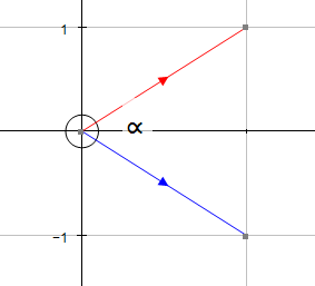
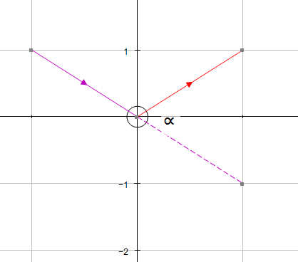
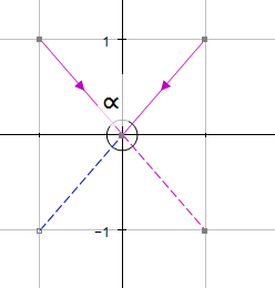
The angle required is always the angle formed when the vectors
are both pointing towards or away from their intersection point.
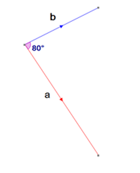
Example
\[
\text{Find the scalar product of vectors }\mathbf{a}\text{ and }\mathbf{b}\text{ if}
\]
\[
\lvert \mathbf{a} \rvert = 4,
\qquad
\lvert \mathbf{b} \rvert = 5,
\qquad
\theta = 80^\circ.
\]
\[
\mathbf{a}\cdot\mathbf{b}
=
\lvert \mathbf{a} \rvert\,\lvert \mathbf{b} \rvert \cos\theta
\]
\[
\mathbf{a}\cdot\mathbf{b}
=
4 \times 5 \times \cos 80^\circ
\]
\[
\mathbf{a}\cdot\mathbf{b}
=
20\cos 80^\circ
\]
\[
\mathbf{a}\cdot\mathbf{b}
=
3.473 \quad (3\text{ d.p.})
\]
Example
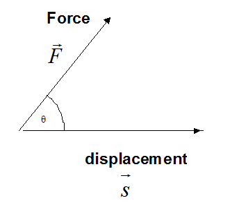
Work done by a constant force:
\[
W
=
\vec{F}\,\cdot\,\vec{s}
\]
Work is scalar, yet force and displacement are vectors.
Power is the rate at which a force does work.
If a force \(F\) does work \(W\) during a time interval \(\Delta t\):
\[
P_{\text{avg}}
=
\frac{W}{\Delta t}
\]
At any particular moment:
\[
P
=
\frac{dW}{dt}
\]
\[
=
\frac{d(Fs)}{dt}
\]
But the force is constant and:
\[
\frac{ds}{dt} = v
\]
So:
\[
P = Fv
\]
If the direction of the force is at an angle θ to the direction of travel:
\[
P = Fv\cos\theta
\]
Then instantaneous power is:
\[
P = \vec{F}\,\cdot\,\vec{v}
\]
Doggo decided to be lazy and accepted a lift from a pleasure boat.
The tow rope exerts a force of 50 N on the kayak
at an angle of 60° to the horizontal.
If the instantaneous power is 100 W,
what is the magnitude of the velocity?
\[
P = \vec{F}\,\cdot\,\vec{v}
\]
\[
P = \lvert F \rvert\,\lvert v \rvert \cos\theta
\]
\[
100 = 50 \cos 60^\circ \,\lvert v \rvert
\]
\[
\lvert v \rvert
=
\frac{100}{50\cos 60^\circ}
\]
\[
\lvert v \rvert = 4
\]
\[
\text{The velocity of the kayak is } 4\text{ m/s.}
\]
Component Form of Dot Product
\[
\text{If }\mathbf{a} =
\begin{pmatrix}
a_1 \\[4pt]
a_2 \\[4pt]
a_3
\end{pmatrix}
\quad\text{and}\quad
\mathbf{b} =
\begin{pmatrix}
b_1 \\[4pt]
b_2 \\[4pt]
b_3
\end{pmatrix}
\]
\[
\text{then }\mathbf{a}\cdot\mathbf{b}
=
a_1 b_1
+
a_2 b_2
+
a_3 b_3
\]
\[
\text{(From the Cosine Rule)}
\]
Example
\[
\text{Find the scalar product of vectors }\mathbf{a}\text{ and }\mathbf{b}\text{ if}
\]
\[
\mathbf{a} =
\begin{pmatrix}
3 \\[4pt]
4
\end{pmatrix},
\qquad
\mathbf{b} =
\begin{pmatrix}
6 \\[4pt]
5
\end{pmatrix}
\]
\[
\mathbf{a}\cdot\mathbf{b}
=
3 \times 6 + 4 \times 5
\]
\[
\mathbf{a}\cdot\mathbf{b}
=
18 + 20
\]
\[
\mathbf{a}\cdot\mathbf{b}
=
38
\]
Example
\[
\text{Find the scalar product of vectors }\mathbf{a}\text{ and }\mathbf{b}\text{ if}
\]
\[
\mathbf{a} =
\begin{pmatrix}
3 \\[4pt]
4 \\[4pt]
5
\end{pmatrix},
\qquad
\mathbf{b} =
\begin{pmatrix}
1 \\[4pt]
-2 \\[4pt]
3
\end{pmatrix}
\]
\[
\mathbf{a}\cdot\mathbf{b}
=
3 \times 1
+
4 \times (-2)
+
5 \times 3
\]
\[
\mathbf{a}\cdot\mathbf{b}
=
3 - 8 + 15
\]
\[
\mathbf{a}\cdot\mathbf{b}
=
10
\]
Place the vectors tail to tail.
\[
\mathbf{a}\cdot\mathbf{b}
=
\lvert \mathbf{a} \rvert\,\lvert \mathbf{b} \rvert \cos\theta
\]
\[
\mathbf{a}\cdot\mathbf{b}
=
a_1 b_1 + a_2 b_2 + a_3 b_3
\]
\[
\text{so }\;
\lvert \mathbf{a} \rvert\,\lvert \mathbf{b} \rvert \cos\theta
=
a_1 b_1 + a_2 b_2 + a_3 b_3
\]
\[
\Rightarrow\quad
\cos\theta
=
\frac{
a_1 b_1 + a_2 b_2 + a_3 b_3
}{
\lvert \mathbf{a} \rvert\,\lvert \mathbf{b} \rvert
}
\]
\[
\Rightarrow\quad
\cos\theta
=
\frac{
\mathbf{a}\cdot\mathbf{b}
}{
\lvert \mathbf{a} \rvert\,\lvert \mathbf{b} \rvert
}
\]
Example
\[
\text{Given position vectors }P(4,3,6)\text{ and }Q(7,3,2),
\]
\[
\text{calculate angle }P\widehat{O}Q\text{.}
\]
\[
\text{Angle }P\widehat{O}Q\text{ is made from }\overrightarrow{OP}\text{ and }\overrightarrow{OQ}.
\]
\[
\text{Let }\mathbf{a} = \overrightarrow{OP}
=
\begin{pmatrix}
4 \\[4pt]
3 \\[4pt]
6
\end{pmatrix}
\quad\text{and}\quad
\mathbf{b} = \overrightarrow{OQ}
=
\begin{pmatrix}
7 \\[4pt]
3 \\[4pt]
2
\end{pmatrix}
\]
\[
\Rightarrow\quad
\cos\theta
=
\frac{\mathbf{a}\cdot\mathbf{b}}{\lvert \mathbf{a} \rvert\,\lvert \mathbf{b} \rvert}
\]
\[
\lvert \overrightarrow{OP} \rvert
=
\sqrt{4^{2} + 3^{2} + 6^{2}}
\]
\[
= \sqrt{16 + 9 + 36}
\]
\[
= \sqrt{61}
\]
\[
\lvert \overrightarrow{OQ} \rvert
=
\sqrt{7^{2} + 3^{2} + 2^{2}}
\]
\[
= \sqrt{49 + 9 + 4}
\]
\[
= \sqrt{62}
\]
\[
\cos\theta
=
\frac{
a_1 b_1 + a_2 b_2 + a_3 b_3
}{
\lvert \mathbf{a} \rvert\,\lvert \mathbf{b} \rvert
}
\]
\[
\Rightarrow\quad
\cos\theta
=
\frac{
4 \times 7 + 3 \times 3 + 6 \times 2
}{
\sqrt{61}\,\times\,\sqrt{62}
}
\]
\[
\Rightarrow\quad
\cos\theta
=
\frac{28 + 9 + 12}{\sqrt{61}\,\times\,\sqrt{62}}
\]
\[
\Rightarrow\quad
\cos\theta
=
\frac{49}{\sqrt{61}\,\times\,\sqrt{62}}
\]
\[
\Rightarrow\quad
\theta
=
\cos^{-1}\!\left(
\frac{49}{\sqrt{61}\,\times\,\sqrt{62}}
\right)
\]
\[
\Rightarrow\quad
\theta \approx 37.177^\circ
\]
Which looks like this:
Example
Calculate the angle θ between vectors:
\[
\mathbf{p}
=
4\mathbf{i}
+
2\mathbf{j}
-
3\mathbf{k}
\quad\text{and}\quad
\mathbf{q}
=
8\mathbf{i}
-
6\mathbf{j}
+
3\mathbf{k}
\]
\[
\mathbf{p}
=
\begin{pmatrix}
4 \\[4pt]
2 \\[4pt]
-3
\end{pmatrix}
\qquad\qquad\qquad
\mathbf{q}
=
\begin{pmatrix}
8 \\[4pt]
-6 \\[4pt]
3
\end{pmatrix}
\]
\[
\lvert \mathbf{p} \rvert
=
\sqrt{4^{2} + 2^{2} + (-3)^{2}}
\]
\[
= \sqrt{16 + 4 + 9}
\]
\[
= \sqrt{29}
\]
\[
\lvert q \rvert
=
\sqrt{8^{2} + (-6)^{2} + 3^{2}}
\]
\[
= \sqrt{64 + 36 + 9}
\]
\[
= \sqrt{109}
\]
\[
\cos\theta
=
\frac{
4 \times 8
+
2 \times (-6)
+
(-3) \times 3
}{
\sqrt{29}\,\times\,\sqrt{109}
}
\]
\[
\Rightarrow\quad
\cos\theta
=
\frac{32 - 12 - 9}{\sqrt{29}\,\times\,\sqrt{109}}
\]
\[
\Rightarrow\quad
\cos\theta
=
\frac{11}{\sqrt{29}\,\times\,\sqrt{109}}
\]
\[
\Rightarrow\quad
\theta
=
\cos^{-1}\!\left(
\frac{11}{\sqrt{29}\,\times\,\sqrt{109}}
\right)
\]
\[
\Rightarrow\quad
\theta \approx 78.717^\circ
\]
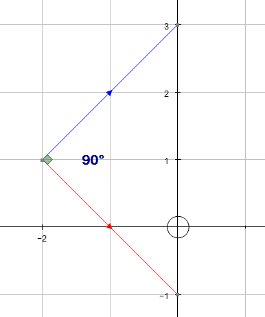
\[
\text{If }\mathbf{a}\text{ and }\mathbf{b}\text{ are perpendicular,}
\]
\[
\mathbf{a}\cdot\mathbf{b} = 0
\]
\[
\text{since }\cos 90^\circ = 0
\]
Example
Triangle ABC has coordinates A(5,7,−5), B(4,7,−3), C(2,7,−4).
Is it right‑angled at B?
\[
\text{Let }\mathbf{a} = \overrightarrow{BA}
=
\begin{pmatrix}
5 \\[4pt]
7 \\[4pt]
-5
\end{pmatrix}
-
\begin{pmatrix}
4 \\[4pt]
7 \\[4pt]
-3
\end{pmatrix}
=
\begin{pmatrix}
1 \\[4pt]
0 \\[4pt]
-2
\end{pmatrix}
\]
\[
\text{and }\mathbf{b} = \overrightarrow{BC}
=
\begin{pmatrix}
2 \\[4pt]
7 \\[4pt]
-4
\end{pmatrix}
-
\begin{pmatrix}
4 \\[4pt]
7 \\[4pt]
-3
\end{pmatrix}
=
\begin{pmatrix}
-2 \\[4pt]
0 \\[4pt]
-1
\end{pmatrix}
\]
\[
\mathbf{a}\cdot\mathbf{b}
=
1 \times (-2)
+
0 \times 0
+
(-2)\times(-1)
\]
\[
\mathbf{a}\cdot\mathbf{b}
=
-2 + 2
\]
\[
\mathbf{a}\cdot\mathbf{b}
=
0
\]
\[
\Rightarrow\;
\mathbf{a}\;\text{and}\;\mathbf{b}\;\text{are perpendicular }(\perp)
\]
\[
\Rightarrow\;
\triangle ABC \text{ is right‑angled at } B
\]
\[
\text{For vectors }\mathbf{a}\text{ and }\mathbf{b}:
\]
\[
\mathbf{a}\cdot\mathbf{b}
=
\mathbf{b}\cdot\mathbf{a}
\]
\[
\text{For vectors }\mathbf{a},\;\mathbf{b},\;\mathbf{c}:
\]
\[
\mathbf{a}\cdot(\mathbf{b}+\mathbf{c})
=
\mathbf{a}\cdot\mathbf{b}
+
\mathbf{a}\cdot\mathbf{c}
\]
More Vectors
Books
Printed resources available at Amazon
These notes are suitable as a revision aid for anyone studying basic vectors.
Topics include:
- Definitions: scalars and vectors
- Column vectors
- Equal vectors
- Magnitude
- Addition of vectors
- Subtraction of vectors
- The zero vector
- Unit vector
- Position vectors
- 3D vectors
- Multiplication of a vector by a scalar
- Section formula
- The scalar (dot) product
- Component form of dot product
- Angle between vectors
- Perpendicular vectors
As an Amazon Associate I earn from qualifying purchases.